This is the most elementary of my favourite formulas. I think I first saw this as a Year 8 student and have been enthralled by it ever since.

In words, the sum of the first N cubes is the square of the sum of the first N squares. Furthermore, both sides are equal to the square of the binomial coefficient 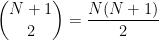 .
.
The formula was discovered by Aryabhata of Patna around 1500 years ago, but it may have been known before then. The most elementary proof is probably one by mathematical induction:
Let S be the set of positive integers N for which  . We wish to show that S is the set of all positive integers
  . Firstly
  since for N=1,
  . Assume
  . That is,

For convenience denote by  the sum
  . Then
![\begin{array}{lcl} \sum_{n=1}^{k+1} n^3 &=& (k+1)^3 + \sum_{n=1}^k n^3\\&=& (k+1)(k+1)^2 + T^2\quad \text{(by the inductive assumption)}\\ &=& T^2 + (k+1)[k(k+1) + (k+1)]\\&=&T^2 + (k+1)[2T + (k+1)]\\ &=& T^2 + 2T(k+1) + (k+1)^2\\&=& (T + (k + 1))^2\\ &=& \left(\sum_{n=1}^{k+1} n \right)^2.\end{array}](https://s0.wp.com/latex.php?latex=%5Cbegin%7Barray%7D%7Blcl%7D+%5Csum_%7Bn%3D1%7D%5E%7Bk%2B1%7D+n%5E3+%26%3D%26+%28k%2B1%29%5E3+%2B+%5Csum_%7Bn%3D1%7D%5Ek+n%5E3%5C%5C%26%3D%26+%28k%2B1%29%28k%2B1%29%5E2+%2B+T%5E2%5Cquad+%5Ctext%7B%28by+the+inductive+assumption%29%7D%5C%5C+%26%3D%26+T%5E2+%2B+%28k%2B1%29%5Bk%28k%2B1%29+%2B+%28k%2B1%29%5D%5C%5C%26%3D%26T%5E2+%2B+%28k%2B1%29%5B2T+%2B+%28k%2B1%29%5D%5C%5C+%26%3D%26+T%5E2+%2B+2T%28k%2B1%29+%2B+%28k%2B1%29%5E2%5C%5C%26%3D%26+%28T+%2B+%28k+%2B+1%29%29%5E2%5C%5C+%26%3D%26+%5Cleft%28%5Csum_%7Bn%3D1%7D%5E%7Bk%2B1%7D+n+%5Cright%29%5E2.%5Cend%7Barray%7D&bg=ffffff&fg=000000&s=0&c=20201002)
This shows that if , then  . Hence by the principle of mathematical induction,
  and we are done.
Next I will show the nicest proof that I am aware of (see p126 of [1] which also contains a proof by picture). We form the grid of numbers of the form  for i and j from 1 to N (as you would see in the multiplication tables) and sum the numbers of the grid in two ways. Below is an example for the case N=5.
| 1 |
|
2 |
|
3 |
|
4 |
|
5 |
|
|
|
|
|
|
|
|
|
| 2 |
|
4 |
|
6 |
|
8 |
|
10 |
|
|
|
|
|
|
|
|
|
| 3 |
|
6 |
|
9 |
|
12 |
|
15 |
|
|
|
|
|
|
|
|
|
| 4 |
|
8 |
|
12 |
|
16 |
|
20 |
|
|
|
|
|
|
|
|
|
| 5 |
|
10 |
|
15 |
|
20 |
|
25 |
The easier sum is simply 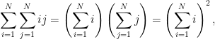 the left side of the formula.
Secondly, we sum along L-shapes, an example of which is shown in bold below.
| 1 |
|
2 |
|
3 |
|
4 |
|
5 |
|
|
|
|
|
|
|
|
|
| 2 |
|
4 |
|
6 |
|
8 |
|
10 |
|
|
|
|
|
|
|
|
|
| 3 |
|
6 |
|
9 |
|
12 |
|
15 |
|
|
|
|
|
|
|
|
|
| 4 |
|
8 |
|
12 |
|
16 |
|
20 |
|
|
|
|
|
|
|
|
|
| 5 |
|
10 |
|
15 |
|
20 |
|
25 |
Note that each number in such an L-shape is a multiple of max(i,j), which ranges from 1 to N. The sum of the numbers in an L-shape is then this multiple times the sum of 1, 2, …, max(i,j)-1, max(i,j), max(i,j) – 1, …, 2, 1, which can easily be shown to be  (think of counting the points of a square grid along diagonals). Hence the total is
 .
.
In other words,
Reference:
[1] C. Alsina and R. Nelsen, “An Invitation to Proofs Without Words”, Eur. J. Pure Appl. Math, 3 (2010), 118-127, available here.

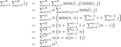
 ) in the context that if measurement errors obey this distribution, then the arithmetic mean of measurements is the optimal estimator in a least squares sense.
 denotes the integral, we have
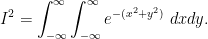
 and
and
![\begin{array}{lcl}I^2 &=& \int_0^{2\pi} \int_0^{\infty} r e^{-r^2}\ dr d\theta\\&=& \int_0^{2\pi}\left[-\frac{1}{2}e^{-r^2} \right]_0^{\infty}\ d\theta\\&=&\int_0^{2\pi}\frac{1}{2}\ d\theta\\&=&\pi,\end{array}](https://s0.wp.com/latex.php?latex=%5Cbegin%7Barray%7D%7Blcl%7DI%5E2+%26%3D%26+%5Cint_0%5E%7B2%5Cpi%7D+%5Cint_0%5E%7B%5Cinfty%7D+r+e%5E%7B-r%5E2%7D%5C+dr+d%5Ctheta%5C%5C%26%3D%26+%5Cint_0%5E%7B2%5Cpi%7D%5Cleft%5B-%5Cfrac%7B1%7D%7B2%7De%5E%7B-r%5E2%7D+%5Cright%5D_0%5E%7B%5Cinfty%7D%5C+d%5Ctheta%5C%5C%26%3D%26%5Cint_0%5E%7B2%5Cpi%7D%5Cfrac%7B1%7D%7B2%7D%5C+d%5Ctheta%5C%5C%26%3D%26%5Cpi%2C%5Cend%7Barray%7D&bg=ffffff&fg=000000&s=0&c=20201002)
 comes in the answer because the Gaussian distribution is rotationally invariant. This distribution pops up in many applications ranging from modelling errors and noise (due to the central limit theorem) to the solution of the heat equation in physics.


